|
AOMedia AV1 Codec
|
|
AOMedia AV1 Codec
|
This document provides an architectural overview of the libaom AV1 encoder.
It is intended as a high level starting point for anyone wishing to contribute to the project, that will help them to more quickly understand the structure of the encoder and find their way around the codebase.
It stands above and will where necessary link to more detailed function level documents.
Most modern video encoders including VP8, H.264, VP9, HEVC and AV1 (in increasing order of complexity) share a common basic paradigm. This comprises separating a stream of raw video frames into a series of discrete blocks (of one or more sizes), then computing a prediction signal and a quantized, transform coded, residual error signal. The prediction and residual error signal, along with any side information needed by the decoder, are then entropy coded and packed to form the encoded bitstream. See Figure 1: below, where the blue blocks are, to all intents and purposes, the lossless parts of the encoder and the red block is the lossy part.
This is of course a gross oversimplification, even in regard to the simplest of the above codecs. For example, all of them allow for block based prediction at multiple different scales (i.e. different block sizes) and may use previously coded pixels in the current frame for prediction or pixels from one or more previously encoded frames. Further, they may support multiple different transforms and transform sizes and quality optimization tools like loop filtering.

As previously stated, AV1 adopts the same underlying paradigm as other block transform based codecs. However, it is much more complicated than previous generation codecs and supports many more block partitioning, prediction and transform options.
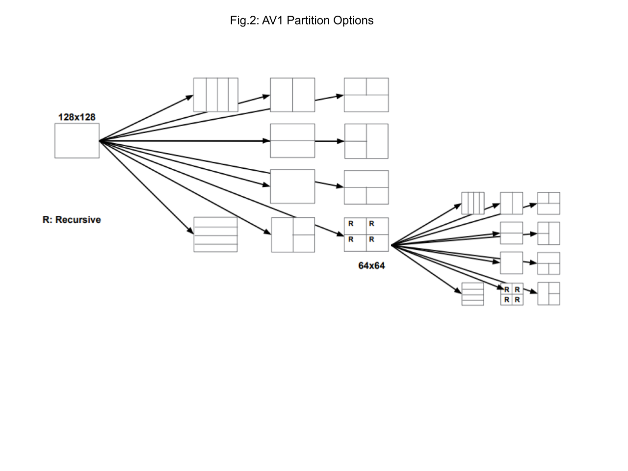
AV1 supports block partitions of various sizes from 128x128 pixels down to 4x4 pixels using a multi-layer recursive tree structure as illustrated in figure 2 below.
AV1 also provides 71 basic intra prediction modes, 56 single frame inter prediction modes (7 reference frames x 4 modes x 2 for OBMC (overlapped block motion compensation)), 12768 compound inter prediction modes (that combine inter predictors from two reference frames) and 36708 compound inter / intra prediction modes. Furthermore, in addition to simple inter motion estimation, AV1 also supports warped motion prediction using affine transforms.
In terms of transform coding, it has 16 separable 2-D transform kernels \((DCT, ADST, fADST, IDTX)^2\) that can be applied at up to 19 different scales from 64x64 down to 4x4 pixels.
When combined together, this means that for any one 8x8 pixel block in a source frame, there are approximately 45,000,000 different ways that it can be encoded.
Consequently, AV1 requires complex control processes. While not necessarily a normative part of the bitstream, these are the algorithms that turn a set of compression tools and a bitstream format specification, into a coherent and useful codec implementation. These may include but are not limited to things like :-
For a more detailed overview of AV1's encoding tools and a discussion of some of the design considerations and hardware constraints that had to be accommodated, please refer to A Technical Overview of AV1.
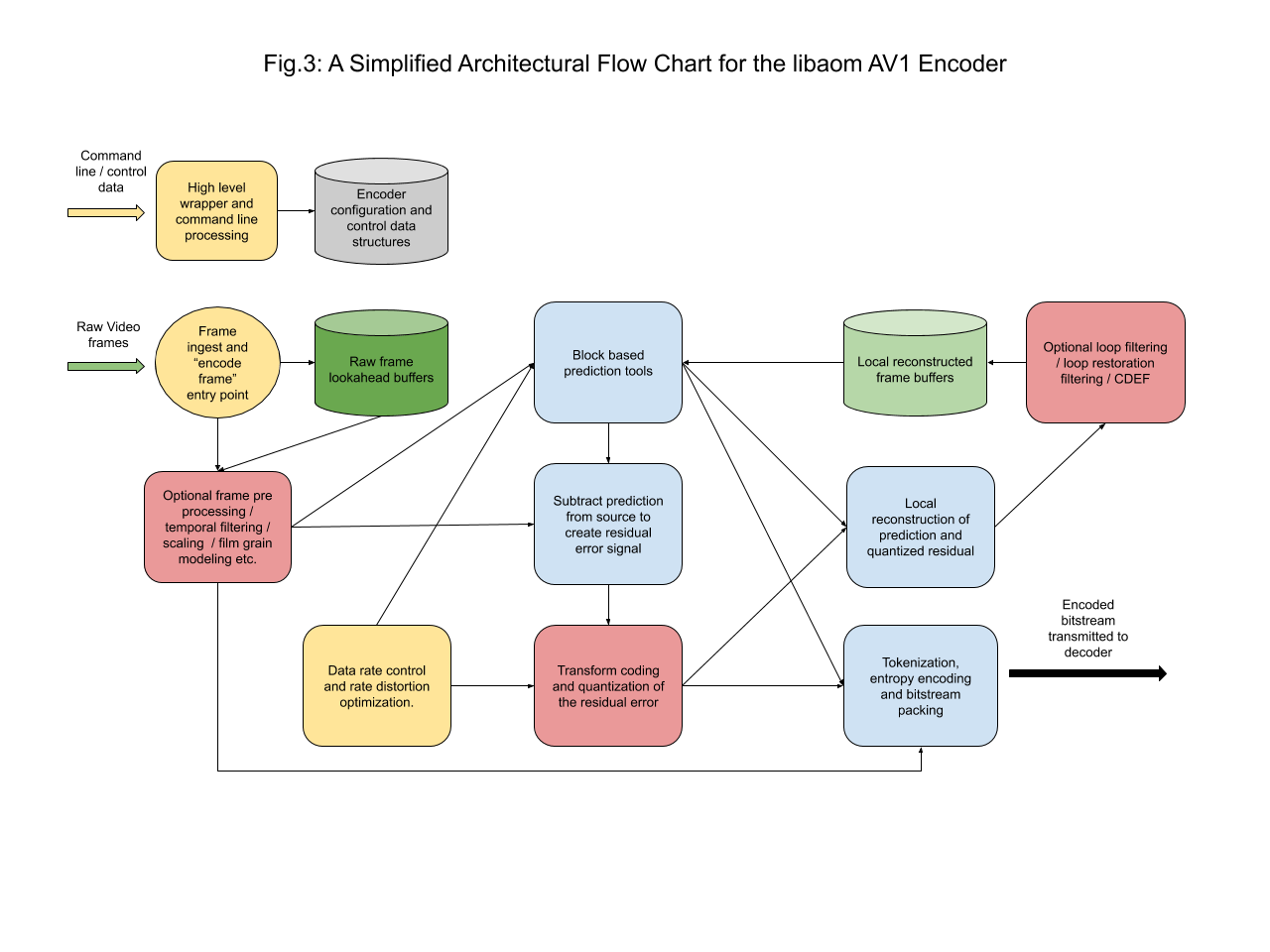
Figure 3 provides a slightly expanded but still simplistic view of the AV1 encoder architecture with blocks that relate to some of the subsequent sections of this document. In this diagram, the raw uncompressed frame buffers are shown in dark green and the reconstructed frame buffers used for prediction in light green. Red indicates those parts of the codec that are (or may be) lossy, where fidelity can be traded off against compression efficiency, whilst light blue shows algorithms or coding tools that are lossless. The yellow blocks represent non-bitstream normative configuration and control algorithms.
Add details or links here: TODO ? elliotk@
The following are the main high level data structures used by the libaom AV1 encoder and referenced elsewhere in this overview document:
The libaom AV1 encoder is configurable to support a number of different use cases and rate control strategies.
The principle use cases for which it is optimised are as follows:
Other examples of use cases for which the encoder could be configured but for which there is less by way of specific optimizations include:
Specific use cases may have particular requirements or constraints. For example:
Video Conferencing: In a video conference we need to encode the video in real time and to avoid any coding tools that could increase latency, such as frame look ahead.
Live Streams: In cases such as live streaming of games or events, it may be possible to allow some limited buffering of the video and use of lookahead coding tools to improve encoding quality. However, whilst a lag of a second or two may be fine given the one way nature of this type of video, it is clearly not possible to use tools such as two pass coding.
Broadcast: Broadcast video (e.g. digital TV over satellite) may have specific requirements such as frequent and regular key frames (e.g. once per second or more) as these are important as entry points to users when switching channels. There may also be strict upper limits on bandwidth over a short window of time.
Download and Play: Download and play applications may have less strict requirements in terms of local frame by frame rate control but there may be a requirement to accurately hit a file size target for the video clip as a whole. Similar considerations may apply to playback from mass storage devices such as DVD or disk drives.
Editing: In certain special use cases such as offline editing, it may be desirable to have very high quality and data rate but also very frequent key frames or indeed to encode the video exclusively as key frames. Lossless video encoding may also be required in this use case.
VOD / Streaming: One of the most important and common use cases for AV1 is video on demand or streaming, for services such as YouTube and Netflix. In this use case it is possible to do two or even multi-pass encoding to improve compression efficiency. Streaming services will often store many encoded copies of a video at different resolutions and data rates to support users with different types of playback device and bandwidth limitations. Furthermore, these services support dynamic switching between multiple streams, so that they can respond to changing network conditions.
Exact rate control when encoding for a specific format (e.g 360P or 1080P on YouTube) may not be critical, provided that the video bandwidth remains within allowed limits. Whilst a format may have a nominal target data rate, this can be considered more as the desired average egress rate over the video corpus rather than a strict requirement for any individual clip. Indeed, in order to maintain optimal quality of experience for the end user, it may be desirable to encode some easier videos or sections of video at a lower data rate and harder videos or sections at a higher rate.
VOD / streaming does not usually require very frequent key frames (as in the broadcast case) but key frames are important in trick play (scanning back and forth to different points in a video) and for adaptive stream switching. As such, in a use case like YouTube, there is normally an upper limit on the maximum time between key frames of a few seconds, but within certain limits the encoder can try to align key frames with real scene cuts.
Whilst encoder speed may not seem to be as critical in this use case, for services such as YouTube, where millions of new videos have to be encoded every day, encoder speed is still important, so libaom allows command line control of the encode speed vs quality trade off.
Fixed Quality / Testing Mode: Libaom also has a fixed quality encoder pathway designed for testing under highly constrained conditions.
In any modern video encoder there are trade offs that can be made in regard to the amount of time spent encoding a video or video frame vs the quality of the final encode.
These trade offs typically limit the scope of the search for an optimal prediction / transform combination with faster encode modes doing fewer partition, reference frame, prediction mode and transform searches at the cost of some reduction in coding efficiency.
The pruning of the size of the search tree is typically based on assumptions about the likelihood of different search modes being selected based on what has gone before and features such as the dimensions of the video frames and the Q value selected for encoding the frame. For example certain intra modes are less likely to be chosen at high Q but may be more likely if similar modes were used for the previously coded blocks above and to the left of the current block.
The speed settings depend both on the use case (e.g. Real Time encoding) and an explicit speed control passed in on the command line as –cpu-used and stored in the AV1_COMP::speed field of the main compressor instance data structure (cpi).
The control flags for the speed trade off are stored the AV1_COMP::sf field of the compressor instancve and are set in the following functions:-
A second factor impacting the speed of encode is rate distortion optimisation (rd vs non-rd encoding).
When rate distortion optimization is enabled each candidate combination of a prediction mode and transform coding strategy is fully encoded and the resulting error (or distortion) as compared to the original source and the number of bits used, are passed to a rate distortion function. This function converts the distortion and cost in bits to a single RD value (where lower is better). This RD value is used to decide between different encoding strategies for the current block where, for example, a one may result in a lower distortion but a larger number of bits.
The calculation of this RD value is broadly speaking as follows:
\[ RD = (λ * Rate) + Distortion \]
This assumes a linear relationship between the number of bits used and distortion (represented by the rate multiplier value λ) which is not actually valid across a broad range of rate and distortion values. Typically, where distortion is high, expending a small number of extra bits will result in a large change in distortion. However, at lower values of distortion the cost in bits of each incremental improvement is large.
To deal with this we scale the value of λ based on the quantizer value chosen for the frame. This is assumed to be a proxy for our approximate position on the true rate distortion curve and it is further assumed that over a limited range of distortion values, a linear relationship between distortion and rate is a valid approximation.
Doing a rate distortion test on each candidate prediction / transform combination is expensive in terms of cpu cycles. Hence, for cases where encode speed is critical, libaom implements a non-rd pathway where the RD value is estimated based on the prediction error and quantizer setting.
The following are the main data structures referenced in this section (see also Main Encoder Data Structures):
To encode a frame, first call av1_receive_raw_frame() to obtain the raw frame data. Then call av1_get_compressed_data() to encode raw frame data into compressed frame data. The main body of av1_get_compressed_data() is av1_encode_strategy(), which determines high-level encode strategy (frame type, frame placement, etc.) and then encodes the frame by calling av1_encode(). In av1_encode(), av1_first_pass() will execute the first_pass of two-pass encoding, while encode_frame_to_data_rate() will perform the final pass for either one-pass or two-pass encoding.
The main body of encode_frame_to_data_rate() is encode_with_recode_loop_and_filter(), which handles encoding before in-loop filters (with recode loops encode_with_recode_loop(), or without any recode loop encode_without_recode()), followed by in-loop filters (deblocking filters loopfilter_frame(), CDEF filters and restoration filters cdef_restoration_frame()).
Except for rate/quality control, both encode_with_recode_loop() and encode_without_recode() call av1_encode_frame() to manage the reference frame buffers and encode_frame_internal() to perform the rest of encoding that does not require access to external frames. encode_frame_internal() is the starting point for the partition search (see Block Partition Search).
Video codecs exploit the spatial and temporal correlations in video signals to achieve compression efficiency. The noise factor in the source signal attenuates such correlation and impedes the codec performance. Denoising the video signal is potentially a promising solution.
One strategy for denoising a source is motion compensated temporal filtering. Unlike image denoising, where only the spatial information is available, video denoising can leverage a combination of the spatial and temporal information. Specifically, in the temporal domain, similar pixels can often be tracked along the motion trajectory of moving objects. Motion estimation is applied to neighboring frames to find similar patches or blocks of pixels that can be combined to create a temporally filtered output.
AV1, in common with VP8 and VP9, uses an in-loop motion compensated temporal filter to generate what are referred to as alternate reference frames (or ARF frames). These can be encoded in the bitstream and stored as frame buffers for use in the prediction of subsequent frames, but are not usually directly displayed (hence they are sometimes referred to as non-display frames).
The following command line parameters set the strength of the filter, the number of frames used and determine whether filtering is allowed for key frames.
Note that in AV1, the temporal filtering scheme is designed around the hierarchical ARF based pyramid coding structure. We typically apply denoising only on key frame and ARF frames at the highest (and sometimes the second highest) layer in the hierarchical coding structure.
Our method divides the current frame into "MxM" blocks. For each block, a motion search is applied on frames before and after the current frame. Only the best matching patch with the smallest mean square error (MSE) is kept as a candidate patch for a neighbour frame. The current block is also a candidate patch. A total of N candidate patches are combined to generate the filtered output.
Let f(i) represent the filtered sample value and \(p_{j}(i)\) the sample value of the j-th patch. The filtering process is:
\[ f(i) = \frac{p_{0}(i) + \sum_{j=1}^{N} ω_{j}(i).p_{j}(i)} {1 + \sum_{j=1}^{N} ω_{j}(i)} \]
where \( ω_{j}(i) \) is the weight of the j-th patch from a total of N patches. The weight is determined by the patch difference as:
\[ ω_{j}(i) = exp(-\frac{D_{j}(i)}{h^2}) \]
where \( D_{j}(i) \) is the sum of squared difference between the current block and the j-th candidate patch:
\[ D_{j}(i) = \sum_{k\inΩ_{i}}||p_{0}(k) - p_{j}(k)||_{2} \]
where:
It is recommended that the reader refers to the code for more details.
The main entry point for temporal filtering is av1_temporal_filter(). This function returns 1 if temporal filtering is successful, otherwise 0. When temporal filtering is applied, the filtered frame will be held in the output_frame, which is the frame to be encoded in the following encoding process.
Almost all temporal filter related code is in av1/encoder/temporal_filter.c and av1/encoder/temporal_filter.h.
Inside av1_temporal_filter(), the reader's attention is directed to tf_setup_filtering_buffer() and tf_do_filtering().
Add details here.
The following are the main data structures referenced in this section (see also Main Encoder Data Structures):
Different use cases (Encoder Use Cases) may have different requirements in terms of data rate control.
The broad rate control strategy is selected using the –end-usage parameter on the command line, which maps onto the field aom_codec_enc_cfg_t::rc_end_usage in aom_encoder.h.
The four supported options are:-
The value of aom_codec_enc_cfg_t::rc_end_usage is in turn copied over into the encoder rate control configuration data structure as RateControlCfg::mode.
In regards to the most important use cases above, Video on demand uses either VBR or CQ mode. CBR is the preferred rate control model for RTC and Live streaming and Fixed Q is only used in testing.
The behaviour of each of these modes is regulated by a series of secondary command line rate control options but also depends somewhat on the selected use case, whether 2-pass coding is enabled and the selected encode speed vs quality trade offs (AV1_COMP::speed and AV1_COMP::sf).
The list below gives the names of the main rate control command line options together with the names of the corresponding fields in the rate control configuration data structures.
The following control aspects of vbr encoding
The following relate to buffer and delay management in one pass low delay and real time coding
For streamed VOD content the most common rate control strategy is Variable Bitrate (VBR) encoding. The CQ mode mentioned above is a variant of this where additional quantizer and quality constraints are applied. VBR encoding may in theory be used in conjunction with either 1-pass or 2-pass encoding.
VBR encoding varies the number of bits given to each frame or group of frames according to the difficulty of that frame or group of frames, such that easier frames are allocated fewer bits and harder frames are allocated more bits. The intent here is to even out the quality between frames. This contrasts with Constant Bitrate (CBR) encoding where each frame is allocated the same number of bits.
Whilst for any given frame or group of frames the data rate may vary, the VBR algorithm attempts to deliver a given average bitrate over a wider time interval. In standard VBR encoding, the time interval over which the data rate is averaged is usually the duration of the video clip. An alternative approach is to target an average VBR bitrate over the entire video corpus for a particular video format (corpus VBR).
The command line for libaom does allow 1 Pass VBR, but this has not been properly optimised and behaves much like 1 pass CBR in most regards, with bits allocated to frames by the following functions:
The main focus here will be on 2-pass VBR encoding (and the related CQ mode) as these are the modes most commonly used for VOD content.
2-pass encoding is selected on the command line by setting –passes=2 (or -p 2).
Generally speaking, in 2-pass encoding, an encoder will first encode a video using a default set of parameters and assumptions. Depending on the outcome of that first encode, the baseline assumptions and parameters will be adjusted to optimize the output during the second pass. In essence the first pass is a fact finding mission to establish the complexity and variability of the video, in order to allow a better allocation of bits in the second pass.
The libaom 2-pass algorithm is unusual in that the first pass is not a full encode of the video. Rather it uses a limited set of prediction and transform options and a fixed quantizer, to generate statistics about each frame. No output bitstream is created and the per frame first pass statistics are stored entirely in volatile memory. This has some disadvantages when compared to a full first pass encode, but avoids the need for file I/O and improves speed.
For two pass encoding, the function av1_encode() will first be called for each frame in the video with the value AV1EncoderConfig::pass = 1. This will result in calls to av1_first_pass().
Statistics for each frame are stored in FIRSTPASS_STATS frame_stats_buf.
After completion of the first pass, av1_encode() will be called again for each frame with AV1EncoderConfig::pass = 2. The frames are then encoded in accordance with the statistics gathered during the first pass by calls to encode_frame_to_data_rate() which in turn calls av1_get_second_pass_params().
In summary the second pass code :-
The main two pass functions in regard to the above include:-
For each frame, the two pass algorithm defines a target number of bits RATE_CONTROL::base_frame_target, which is then adjusted if necessary to reflect any undershoot or overshoot on previous frames to give RATE_CONTROL::this_frame_target.
As well as RATE_CONTROL::active_worst_quality, the two pass code also maintains a record of the actual Q value used to encode previous frames at each level in the current pyramid hierarchy (PRIMARY_RATE_CONTROL::active_best_quality). The function rc_pick_q_and_bounds(), uses these values to set a permitted Q range for each frame.
1 pass lagged encode falls between simple 1 pass encoding and full two pass encoding and is used for cases where it is not possible to do a full first pass through the entire video clip, but where some delay is permissible. For example near live streaming where there is a delay of up to a few seconds. In this case the first pass and second pass are in effect combined such that the first pass starts encoding the clip and the second pass lags behind it by a few frames. When using this method, full sequence level statistics are not available, but it is possible to collect and use frame or group of frame level data to help in the allocation of bits and in defining ARF/GF coding hierarchies. The reader is referred to the AV1_PRIMARY::lap_enabled field in the main compressor instance (where lap stands for look ahead processing). This encoding mode for the most part uses the same rate control pathways as two pass VBR encoding.
Having established a target rate for a given frame and an allowed range of Q values, the encoder then tries to encode the frame at a rate that is as close as possible to the target value, given the Q range constraints.
There are two main mechanisms by which this is achieved.
The first selects a frame level Q, using an adaptive estimate of the number of bits that will be generated when the frame is encoded at any given Q. Fundamentally this mechanism is common to VBR, CBR and to use cases such as RTC with small adjustments.
As the Q value mainly adjusts the precision of the residual signal, it is not actually a reliable basis for accurately predicting the number of bits that will be generated across all clips. A well predicted clip, for example, may have a much smaller error residual after prediction. The algorithm copes with this by adapting its predictions on the fly using a feedback loop based on how well it did the previous time around.
The main functions responsible for the prediction of Q and the adaptation over time, for the two pass encoding pipeline are:
A second mechanism for control comes into play if there is a large rate miss for the current frame (much too big or too small). This is a recode mechanism which allows the current frame to be re-encoded one or more times with a revised Q value. This obviously has significant implications for encode speed and in the case of RTC latency (hence it is not used for the RTC pathway).
Whether or not a recode is allowed for a given frame depends on the selected encode speed vs quality trade off. This is set on the command line using the –cpu-used parameter which maps onto the AV1_COMP::speed field in the main compressor instance data structure.
The value of AV1_COMP::speed, combined with the use case, is used to populate the speed features data structure AV1_COMP.sf. In particular HIGH_LEVEL_SPEED_FEATURES::recode_loop determines the types of frames that may be recoded and HIGH_LEVEL_SPEED_FEATURES::recode_tolerance is a rate error trigger threshold.
For more information the reader is directed to the following functions:
There are two main fixed Q cases:
The reader is also refered to the following functions:
The following are the main data structures referenced in this section (see also Main Encoder Data Structures):
To process a sequence/stream of video frames, the encoder divides the frames into groups and encodes them sequentially (possibly dependent on previous groups). In AV1 such a group is usually referred to as a golden frame group (GF group) or sometimes an Alt-Ref (ARF) group or a group of pictures (GOP). A GF group determines and stores the coding structure of the frames (for example, frame type, usage of the hierarchical structure, usage of overlay frames, etc.) and can be considered as the base unit to process the frames, therefore playing an important role in the encoder.
The length of a specific GF group is arguably the most important aspect when determining a GF group. This is because most GF group level decisions are based on the frame characteristics, if not on the length itself directly. Note that the GF group is always a group of consecutive frames, which means the start and end of the group (so again, the length of it) determines which frames are included in it and hence determines the characteristics of the GF group. Therefore, in this document we will first discuss the GF group length decision in Libaom, followed by frame structure decisions when defining a GF group with a certain length.
The basic intuition of determining the GF group length is that it is usually desirable to group together frames that are similar. Hence, we may choose longer groups when consecutive frames are very alike and shorter ones when they are very different.
The determination of the GF group length is done in function calculate_gf_length(). The following encoder use cases are supported:
Single pass with look-ahead disabled(has_no_stats_stage()): in this case there is no information available on the following stream of frames, therefore the function will set the GF group length for the current and the following GF groups (a total number of MAX_NUM_GF_INTERVALS groups) to be the maximum value allowed.
Single pass with look-ahead enabled (AV1_PRIMARY::lap_enabled): look-ahead processing is enabled for single pass, therefore there is a limited amount of information available regarding future frames. In this case the function will determine the length based on FIRSTPASS_STATS (which is generated when processing the look-ahead buffer) for only the current GF group.
Except for the first trivial case where there is no prior knowledge of the following frames, the function calculate_gf_length() tries to determine the GF group length based on the first pass statistics. The determination is divided into two parts:
Baseline decision based on accumulated statistics: this part of the function iterates through the firstpass statistics of the following frames and accumulates the statistics with function accumulate_next_frame_stats. The accumulated statistics are then used to determine whether the correlation in the GF group has dropped too much in function detect_gf_cut. If detect_gf_cut returns non-zero, or if we've reached the end of first-pass statistics, the baseline decision is set at the current point.
As mentioned, for two-pass encoding, the function calculate_gf_length() tries to determine the length of as many as MAX_NUM_GF_INTERVALS groups. The decisions are stored in PRIMARY_RATE_CONTROL::gf_intervals[]. The variables RATE_CONTROL::intervals_till_gf_calculate_due and PRIMARY_RATE_CONTROL::gf_intervals[] help with managing and updating the stored decisions. In the function define_gf_group(), the corresponding stored length decision will be used to define the current GF group.
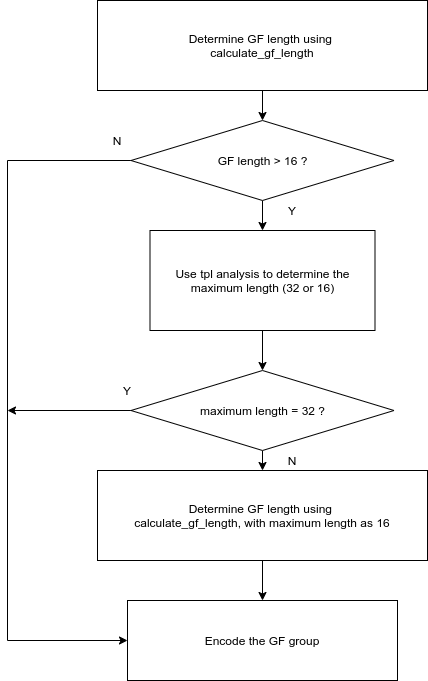
When the maximum GF group length is larger or equal to 32, the encoder will enforce an extra layer to determine whether to use maximum GF length of 32 or 16 for every GF group. In such a case, calculate_gf_length() is first called with the original maximum length (>=32). Afterwards, av1_tpl_setup_stats() is called to analyze the determined GF group and compare the reference to the last frame and the middle frame. If it is decided that we should use a maximum GF length of 16, the function calculate_gf_length() is called again with the updated maximum length, and it only sets the length for a single GF group (RATE_CONTROL::intervals_till_gf_calculate_due is set to 1). This process is shown below.
Before encoding each frame, the encoder checks RATE_CONTROL::frames_till_gf_update_due. If it is zero, indicating processing of the current GF group is done, the encoder will check whether RATE_CONTROL::intervals_till_gf_calculate_due is zero. If it is, as discussed above, calculate_gf_length() is called with original maximum length. If it is not zero, then the GF group length value stored in PRIMARY_RATE_CONTROL::gf_intervals[PRIMARY_RATE_CONTROL::cur_gf_index] is used (subject to change as discussed above).
The function define_gf_group() defines the frame structure as well as other GF group level parameters (e.g. bit allocation) once the length of the current GF group is determined.
The function first iterates through the first pass statistics in the GF group to accumulate various stats, using accumulate_this_frame_stats() and accumulate_next_frame_stats(). The accumulated statistics are then used to determine the use of the use of ALTREF frame along with other properties of the GF group. The values of PRIMARY_RATE_CONTROL::cur_gf_index, RATE_CONTROL::intervals_till_gf_calculate_due and RATE_CONTROL::frames_till_gf_update_due are also updated accordingly.
The function av1_gop_setup_structure() is called at the end to determine the frame layers and reference maps in the GF group, where the construct_multi_layer_gf_structure() function sets the frame update types for each frame and the group structure.
As mentioned, the encoder may use Temporal dependancy modelling (TPL - see Temporal Dependency Modelling) to determine whether we should use a maximum length of 32 or 16 for the current GF group. This requires calls to define_gf_group() but should not change other settings (since it is in essence a trial). This special case is indicated by the setting parameter is_final_pass for to zero.
For single pass encodes where look-ahead processing is disabled (AV1_PRIMARY::lap_enabled = 0), define_gf_group_pass0() is used instead of define_gf_group().
A special constraint for GF group length is the location of the next keyframe (KF). The frames between two KFs are referred to as a KF group. Each KF group can be encoded and decoded independently. Because of this, a GF group cannot span beyond a KF and the location of the next KF is set as a hard boundary for GF group length.
For two-pass encoding RATE_CONTROL::frames_to_key controls when to encode a key frame. When it is zero, the current frame is a keyframe and the function find_next_key_frame() is called. This in turn calls define_kf_interval() to work out where the next key frame should be placed.
For single-pass with look-ahead enabled, define_kf_interval() is called whenever a GF group update is needed (when RATE_CONTROL::frames_till_gf_update_due is zero). This is because generally KFs are more widely spaced and the look-ahead buffer is usually not long enough.
The function define_kf_interval() tries to detect a scenecut. If a scenecut within kf-max-dist is detected, then it is set as the next keyframe. Otherwise the given maximum value is used.
The temporal dependency model runs at the beginning of each GOP. It builds the motion trajectory within the GOP in units of 16x16 blocks. The temporal dependency of a 16x16 block is evaluated as the predictive coding gains it contributes to its trailing motion trajectory. This temporal dependency model reflects how important a coding block is for the coding efficiency of the overall GOP. It is hence used to scale the Lagrangian multiplier used in the rate-distortion optimization framework.
The temporal dependency model and its applications are by default turned on in libaom encoder for the VoD use case. To disable it, use –tpl-model=0 in the aomenc configuration.
The scheme works in the reverse frame processing order over the source frames, propagating information from future frames back to the current frame. For each frame, a propagation step is run for each MB. it operates as follows:
Estimate the intra prediction cost in terms of sum of absolute Hadamard transform difference (SATD) noted as intra_cost. It also loads the motion information available from the first-pass encode and estimates the inter prediction cost as inter_cost. Due to the use of hybrid inter/intra prediction mode, the inter_cost value is further upper bounded by intra_cost. A propagation cost variable is used to collect all the information flowed back from future processing frames. It is initialized as 0 for all the blocks in the last processing frame in a group of pictures (GOP).
The fraction of information from a current block to be propagated towards its reference block is estimated as:
\[ propagation\_fraction = (1 - inter\_cost/intra\_cost) \]
It reflects how much the motion compensated reference would reduce the prediction error in percentage.
The total amount of information the current block contributes to the GOP is estimated as intra_cost + propagation_cost. The information that it propagates towards its reference block is captured by:
\[ propagation\_amount = (intra\_cost + propagation\_cost) * propagation\_fraction \]
Note that the reference block may not necessarily sit on the grid of 16x16 blocks. The propagation amount is hence dispensed to all the blocks that overlap with the reference block. The corresponding block in the reference frame accumulates its own propagation cost as it receives back propagation.
\[ propagation\_cost = propagation\_cost + (\frac{overlap\_area}{(16*16)} * propagation\_amount) \]
In the final encoding stage, the distortion propagation factor of a block is evaluated as \((1 + \frac{propagation\_cost}{intra\_cost})\), where the second term captures its impact on later frames in a GOP.
The Lagrangian multiplier is adapted at the 64x64 block level. For every 64x64 block in a frame, we have a distortion propagation factor:
\[ dist\_prop[i] = 1 + \frac{propagation\_cost[i]}{intra\_cost[i]} \]
where i denotes the block index in the frame. We also have the frame level distortion propagation factor:
\[ dist\_prop = 1 + \frac{\sum_{i}propagation\_cost[i]}{\sum_{i}intra\_cost[i]} \]
which is used to normalize the propagation factor at the 64x64 block level. The Lagrangian multiplier is hence adapted as:
\[ λ[i] = λ[0] * \frac{dist\_prop}{dist\_prop[i]} \]
where λ0 is the multiplier associated with the frame level QP. The 64x64 block level QP is scaled according to the Lagrangian multiplier.
The reader is also refered to the following functions and data structures:
A frame is first split into tiles in encode_tiles(), with each tile compressed by av1_encode_tile(). Then a tile is processed in superblock rows via av1_encode_sb_row() and then encode_sb_row().
The partition search processes superblocks sequentially in encode_sb_row(). Two search modes are supported, depending upon the encoding configuration, encode_nonrd_sb() is for 1-pass and real-time modes, while encode_rd_sb() performs more exhaustive rate distortion based searches.
Partition search over the recursive quad-tree space is implemented by recursive calls to av1_nonrd_use_partition(), av1_rd_use_partition(), or av1_rd_pick_partition() and returning best options for sub-trees to their parent partitions.
In libaom, the partition search lays on top of the mode search (predictor, transform, etc.), instead of being a separate module. The interface of mode search is pick_sb_modes(), which connects the partition_search with Inter Prediction Mode Search and Intra Mode Search. To make good decisions, reconstruction is also required in order to build references and contexts. This is implemented by encode_sb() at the sub-tree level and encode_b() at coding block level.
See also Partition Search
AV1 also provides 71 different intra prediction modes, i.e. modes that predict only based upon information in the current frame with no dependency on previous or future frames. For key frames, where this independence from any other frame is a defining requirement and for other cases where intra only frames are required, the encoder need only considers these modes in the rate distortion loop.
Even so, in most use cases, searching all possible intra prediction modes for every block and partition size is not practical and some pruning of the search tree is necessary.
For the Rate distortion optimized case, the main top level function responsible for selecting the intra prediction mode for a given block is av1_rd_pick_intra_mode_sb(). The readers attention is also drawn to the functions hybrid_intra_mode_search() and av1_nonrd_pick_intra_mode() which may be used where encode speed is critical. The choice between the rd path and the non rd or hybrid paths depends on the encoder use case and the AV1_COMP::speed parameter. Further fine control of the speed vs quality trade off is provided by means of fields in AV1_COMP::sf (which has type SPEED_FEATURES).
Note that some intra modes are only considered for specific use cases or types of video. For example the palette based prediction modes are often valueable for graphics or screen share content but not for natural video. (See av1_search_palette_mode())
See also Intra Mode Search for more details.
For inter frames, where we also allow prediction using one or more previously coded frames (which may chronologically speaking be past or future frames or non-display reference buffers such as ARF frames), the size of the search tree that needs to be traversed, to select a prediction mode, is considerably more massive.
In addition to the 71 possible intra modes we also need to consider 56 single frame inter prediction modes (7 reference frames x 4 modes x 2 for OBMC (overlapped block motion compensation)), 12768 compound inter prediction modes (these are modes that combine inter predictors from two reference frames) and 36708 compound inter / intra prediction modes.
As with the intra mode search, libaom supports an RD based pathway and a non rd pathway for speed critical use cases. The entry points for these two cases are av1_rd_pick_inter_mode() and av1_nonrd_pick_inter_mode_sb() respectively.
Various heuristics and predictive strategies are used to prune the search tree with fine control provided through the speed features parameter in the main compressor instance data structure AV1_COMP::sf.
It is worth noting, that some prediction modes incurr a much larger rate cost than others (ignoring for now the cost of coding the error residual). For example, a compound mode that requires the encoder to specify two reference frames and two new motion vectors will almost inevitable have a higher rate cost than a simple inter prediction mode that uses a predicted or 0,0 motion vector. As such, if we have already found a mode for the current block that has a low RD cost, we can skip a large number of the possible modes on the basis that even if the error residual is 0 the inherent rate cost of the mode itself will garauntee that it is not chosen.
See also Inter Mode Search for more details.
AV1 implements the transform stage using 4 seperable 1-d transforms (DCT, ADST, FLIPADST and IDTX, where FLIPADST is the reversed version of ADST and IDTX is the identity transform) which can be combined to give 16 2-d combinations.
These combinations can be applied at 19 different scales from 64x64 pixels down to 4x4 pixels.
This gives rise to a large number of possible candidate transform options for coding the residual error after prediction. An exhaustive rate-distortion based evaluation of all candidates would not be practical from a speed perspective in a production encoder implementation. Hence libaom addopts a number of strategies to prune the selection of both the transform size and transform type.
There are a number of strategies that have been tested and implememnted in libaom including:
TODO Add link to paper when available
See also Transform Search for more details.
AV1 supports three types of post encode in loop filtering to improve the quality of the reconstructed video.
VP9, used a binary arithmetic coder to encode symbols, where the propability of a 1 or 0 at each descision node was based on a context model that took into account recently coded values (for example previously coded coefficients in the current block). A mechanism existed to update the context model each frame, either explicitly in the bitstream, or implicitly at both the encoder and decoder based on the observed frequency of different outcomes in the previous frame. VP9 also supported seperate context models for different types of frame (e.g. inter coded frames and key frames).
In contrast, AV1 uses an M-ary symbol arithmetic coder to compress the syntax elements, where integer \(M\in[2, 14]\). This approach is based upon the entropy coding strategy used in the Daala video codec and allows for some bit-level parallelism in its implementation. AV1 also has an extended context model and allows for updates to the probabilities on a per symbol basis as opposed to the per frame strategy in VP9.
To improve the performance / throughput of the arithmetic encoder, especially in hardware implementations, the probability model is updated and maintained at 15-bit precision, but the arithmetic encoder only uses the most significant 9 bits when encoding a symbol. A more detailed discussion of the algorithm and design constraints can be found in A Technical Overview of AV1.
TODO add references to key functions / files.
As with VP9, a mechanism exists in AV1 to encode some elements into the bitstream as uncrompresed bits or literal values, without using the arithmetic coder. For example, some frame and sequence header values, where it is beneficial to be able to read the values directly.
TODO add references to key functions / files.
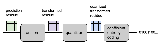
Transform coefficient coding is where the encoder compresses a quantized version of prediction residue into the bitstream.
Before the entropy coding stage, the encoder decouple the pixel-to-pixel correlation of the prediction residue by transforming the residue from the spatial domain to the frequency domain. Then the encoder quantizes the transform coefficients to make the coefficients ready for entropy coding.
The encoder uses av1_write_coeffs_txb() to write the coefficients of a transform block into the bitstream. The coding process has three stages.
Related functions:
To improve the compression efficiency, the encoder uses several context models tailored for transform coefficients to capture the correlations between coding symbols. Most of the context models are built to capture the correlations between the coefficients within the same transform block. However, transform block skip flag (txb_skip) and the sign of dc coefficient (dc_sign) require context info from neighboring transform blocks.
Here is how context info spread between transform blocks. Before coding a transform block, the encoder will use get_txb_ctx() to collect the context information from neighboring transform blocks. Then the context information will be used for coding transform block skip flag (txb_skip) and the sign of dc coefficient (dc_sign). After the transform block is coded, the encoder will extract the context info from the current block using av1_get_txb_entropy_context(). Then encoder will store the context info into a byte (uint8_t) using av1_set_entropy_contexts(). The encoder will use the context info to code other transform blocks.
Related functions:
Beside the actual entropy coding, the encoder uses several utility functions to make optimal RD decisions.
The encoder uses av1_cost_coeffs_txb() or av1_cost_coeffs_txb_laplacian() to estimate the entropy cost of a transform block. Note that av1_cost_coeffs_txb() is slower but accurate whereas av1_cost_coeffs_txb_laplacian() is faster but less accurate.
Related functions:
Beside computing entropy cost, the encoder also uses av1_optimize_txb() to adjust the coefficient’s quantized levels to achieve optimal RD trade-off. In av1_optimize_txb(), the encoder goes through each quantized coefficient and lowers the quantized coefficient level by one if the action yields a better RD score.
Related functions:
All the related functions are listed in Transform Coefficient Coding and Optimization.
In order to efficiently encode video on modern platforms, it is necessary to implement optimized versions of many core encoding and decoding functions using architecture-specific SIMD instructions.
Functions which have optimized implementations will have multiple variants in the code, each suffixed with the name of the appropriate instruction set. There will additionally be an _c version, which acts as a reference implementation which the SIMD variants can be tested against.
As different machines with the same nominal architecture may support different subsets of SIMD instructions, we have dynamic CPU detection logic which chooses the appropriate functions to use at run time. This process is handled by build/cmake/rtcd.pl, with function definitions in the files *_rtcd_defs.pl elsewhere in the codebase.
Currently SIMD is supported on the following platforms:
We aim to provide implementations of all performance-critical functions which are compatible with the instruction sets listed above. Additional SIMD extensions (e.g. AVX on x86, SVE on Arm) are also used to provide even greater performance where available.